Lock your doors, board up the windows, and prepare yourself for a deeper look into PID loops! Now, if you are still here, great! If you ran out of the room screaming like I did, you can catch up later. For some, PID loops can be scary. After all, they are pretty complex and involve CALCULUS. Hold on, I think I’m gonna turn on all the lights real quick… ok, that’s better. PID loops shouldn’t be something to fear; they can be confusing but they are not impossible.
What is a PID Loop?

PID is an acronym for Proportional, Integral and Derivative. It is a control function that is frequently used in process control. You take a reference signal in from your process, compare it to your setpoint, and then change the output to the control device accordingly to minimize the error. Think of the cruise control in your car. You set the speed you want to travel at, your car’s computer will compare that to the current speed, and either accelerate or decelerate to match that setpoint and remove the error. The bigger the error, the bigger the gain or response. For example, when your car on cruise control revs the engine when you start up a hill, the error between the setpoint and the current speed increased so much that the response was also greatly increased.
ALERT: Calculus Ahead!
WARNING: Readers with sensitivity to math equations, including integral-induced headaches, differential skin rashes or anyone who has had prior calculus-related trauma of any kind, should avert their eyes and not proceed any further.
To help us better understand how a PID loop works, let’s take a closer look at a PID equation:

Stay with me, stay with me, it’s not as bad as it looks. We’ll take it in pieces:
![]() represents the control output at the moment of time “n”. This is the amount of gain or response sent to the control device.
represents the control output at the moment of time “n”. This is the amount of gain or response sent to the control device.
![]() is the calculated error at the moment of time “n”. It is calculated by subtracting the current value from the set point.
is the calculated error at the moment of time “n”. It is calculated by subtracting the current value from the set point.
![]() is the Proportional Term (P) of the PID equation. Kc is the proportional gain coefficient and is a fixed value.
is the Proportional Term (P) of the PID equation. Kc is the proportional gain coefficient and is a fixed value.
![]() is the Integral Term (I) of the PID equation and the most frightening. It is simply the sum of the calculated errors from the first sample ( i=1 ) to the current moment “n”. This sum is then multiplied by the Integral coefficient Ki which is calculated using the formula: Ki = Kc * (sample rate/integral time). Basically, the integral coefficient is the proportional coefficient times the ratio of sample rate to integral time. It will make sense once we start plugging in values….I hope.
is the Integral Term (I) of the PID equation and the most frightening. It is simply the sum of the calculated errors from the first sample ( i=1 ) to the current moment “n”. This sum is then multiplied by the Integral coefficient Ki which is calculated using the formula: Ki = Kc * (sample rate/integral time). Basically, the integral coefficient is the proportional coefficient times the ratio of sample rate to integral time. It will make sense once we start plugging in values….I hope.
![]() is the Derivative Term (D) of the PID equation. All you do here is subtract the error found at the previous sample (en-1) from the error now (en) and multiply it by the calculated derivative coefficient. The derivative coefficient is calculated using the formula: Kr = Kc * (derivative time/sample rate). Mathematically, the derivative term will look at the difference between the error now and the error before, determine how rapidly the process variable is deviating from or correcting to the setpoint and adjust the output accordingly. Simple, right?
is the Derivative Term (D) of the PID equation. All you do here is subtract the error found at the previous sample (en-1) from the error now (en) and multiply it by the calculated derivative coefficient. The derivative coefficient is calculated using the formula: Kr = Kc * (derivative time/sample rate). Mathematically, the derivative term will look at the difference between the error now and the error before, determine how rapidly the process variable is deviating from or correcting to the setpoint and adjust the output accordingly. Simple, right?
![]() represents the initial control output when the loop is activated. If transitioning from a manual operation, this value is transferred when the loop transitions to auto mode.
represents the initial control output when the loop is activated. If transitioning from a manual operation, this value is transferred when the loop transitions to auto mode.
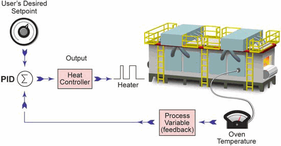
So, now that you know all of the pieces and what they do, you need to know how they fit together. The best way to do that is with an example. So, let’s apply the equation to a temperature control loop. In our example, the loop is maintaining the temperature of an oven, as seen below, and the desired temperature of the oven is 350°F.

For this particular application, we will set the equation’s parameters as follows:
- Kr = 0 (To achieve this, set the Derivative Time to zero. This will make the loop a PI controller; we will look at the derivative reaction later.)
- Kc = 3 (Proportional Gain)
- Ts = 60 seconds (Sample Rate)
- Ki = 1 (To achieve this, set the Integral Time to 180 seconds, Ki = Kc * (sample rate/integral time) or Ki = 3*60/180 = 1
- M(0) = 30 (Initial Control Output)
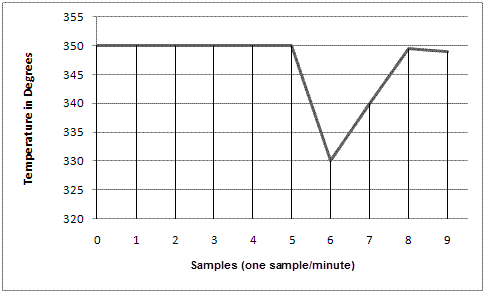
The following graph shows the temperature fluctuation over the past 9 minutes. Let’s see how the equation operates.

At sample zero, the loop has an initial control output (M(0)) of 30. Looking at the graph we can see that with this control output the loop has been stable at 350°F for the first five samples. After the fifth sample, something occurs to make the temperature drop 20°F. This is seen in our actual temperature reading at sample six. Therefore, the error in the system at sample six is calculated to be: e(6) = setpoint – current value = 350 – 330 = 20. Also, at this point we can easily calculate the sum of all the errors for the system:

= (e(1) + e(2) + e(3) + e(4) + e(5) + e(6)) = (0+0+0+0+0+20) = 20.
So using the parameters and calculated values above, the equation for the loop at sample six would become: (colors represent proportional, integral and derivative terms)

M(6) = (3 * 20) + (1 * 20) + (0 * (20-0)) + 30
M(6) = 60 + 20 + 0 + 30
M(6) = 110
At this point, there is an increase in the control output of 80 from the initial control output, and the proportional term is the main force driving this increase with a value of 60. This control output will be converted to an analog value (0-10V, 4-20mA, etc.) that is fed to an end device. In our example, that device is the heating element inside an industrial oven. As the control output drives the temperature toward the setpoint, we see, at sample seven, that the error has decreased to: e(7) = SP-CV = 350 – 340 = 10. Also at this point, the sum of all the sample errors will equal 30 ((e(1) + e(2) + e(3) + e(4) + e(5) + e(6) + e(7)) = (0+0+0+0+0+20+10) = 30) and the equation will become:
M(7) = (3 * 10) + (1 * 30) + (0 * (10-20)) + 30
M(7) = 30 + 30 + 0 + 30
M(7) = 90
Here we see that as the error is corrected, the control output will decrease due to the drop in the proportional term. However, notice that the integral term has risen slightly. At sample eight, the oven temperature has recovered to 349.5°F leaving a minimal error of: e(8) = SP-CV = 350 – 349.5 = 0.5. The sum of all sample errors is now 30.5 and the control output equals:
M(8) = (3 * 0.5) + (1 * 30.5) + (0*(0.5-10)) + 30
M(8) = 1.5 + 30.5 + 0 + 30
M(8) = 61.5
At this point, the proportional term has dropped off considerably and the integral bias has exceeded the proportional gain in controlling the output. You can see that across the three samples the proportional term has gone from 60 to 30 to 1.5 as the error decreases, while the integral term has gone from 20 to 30 to 30.5. When tuning a loop, it is important to remember that with large errors the proportional term will drive the output and with small errors the integral term will take control.
Wow, you’ve made it this far and I am proud of you! For your reward we will now look at the derivative term and how it affects the equation. Wait, where you going?…The job of the derivative term is to keep stability in the loop. With our example, the rate of change is very rapid at sample six – a 20°F drop within one minute. With very rapid changes, there is a risk of instability and the derivative term attempts to alleviate this while aiding in the correction. As mentioned previously, the derivative term will look at the difference between the error now and the error before, determine how rapidly the process variable is deviating from or correcting to the setpoint and adjust the output accordingly.
If we add a derivative coefficient of Kr = 1 (set the Derivative Time (Td) to 20 seconds, Kr = Kc * (derivative time/sample rate) or Kr = 3*20/60 = 1) to the samples in our discussion they become:
M(6) = (3 * 20) + (1 * 20) + (1 * (20-0)) + 30
M(6) = 60 + 20 + 20 + 30
M(6) = 130
M(7) = (3 * 10) + (1 * 30) + (1 * (10-20)) + 30
M(7) = 30 + 30 – 10 + 30
M(7) = 80
M(8) = (3 * 0.5) + (1 * 30.5) + (1 * (0.5-10)) + 30
M(8) = 1.5 + 30.5 – 9.5 + 30
M(8) = 52.5
Looking at the samples above you can see that after our dramatic temperature drop at sample six, the derivative term starts to lessen the control output at sample seven, going from a +20 gain in sample M(6) to a -10 in sample M(7). At this point, the derivative term determined that the process variable was approaching the setpoint at a very rapid rate and dampened the control output to avoid an overshoot of the setpoint.
Well, there you have it, the basics of PID control. PID loops are very important in industrial automation and aren’t something you should be intimidated by. Yes they are complex, and yes they use calculus but they really aren’t too bad. The built-in function blocks in some PLC ladder logic instruction sets can do the heavy calculation lifting for you; the most important tasks then are choosing the coefficient values and tuning the loop for maximum control and performance. Hopefully knowing what each term means and how they affect the equation will help you understand how to set them up. If you would like to see some informative videos on how to use PID loops, check out our Cookbook Series on PID.


