Fiber optic sensors work well in tight spots and in applications with a high degree of electrical noise, but care must be taken when specifying these critical components.
Sensing part presence in machines, in fixtures and on conveyors is an important part of industrial automation. Error proofing assembly and controlling sequence based on presence or absence of a part is often required. In many cases, one can’t just assume the part is where it should be or the nest is empty as expected, so a presence sensor must be used for verification.
There are many types of sensors on the market including inductive, magnetic, capacitive and photoelectric. Each has its own strengths and weaknesses depending on the application. Photoelectric sensors, however, have the broadest offering of types and technologies, and the widest range of applications.
Photoelectric sensors come with a variety of light emission types (infrared, visible red, laser Class 1 and 2), sensing technologies (diffuse, background suppression, reflective, through-beam), and housing configurations (photo eye or fiber optic). This article focuses on specifying and applying fiber optic sensors as they provide advanced capabilities and configuration options, and are great for tight spots where a photo eye sensor won’t fit.
Fiber Optic Technology
Fiber optic sensors, sometimes called fiber photoelectric sensors, include two devices which are typically specified separately: the amplifier, often called the electronics or fiber photoelectric amplifier; and the fiber optic cable, which includes the optic sensor head and the fiber cable which transmits light to and from the amplifier.
The basic theory behind all photoelectric sensors is quite simple. Every photo eye has a light emitter producing the source signal and a receiver which looks for the source signal. There are many different technologies for sensing and measuring the light transmitted to the receiver. For example, background suppression sensors look for the angle at which the light is returned, while standard photo eyes look for the amount of light, called excess gain, returned to the sensor. Other sensors monitor the time light takes to return to provide distance measurement.
Photo eyes contain the emitter and receiver in either one optical sensor head such as used in diffuse and reflective units, or two optical sensor heads as used in through-beam units. Fiber optic sensors have all the electronics in a single housing, with the optical heads for the emitter and receiver separated from and connected to the electronics housing via a fiber cable. The emitted and received light travels through these fiber cables, much like high speed data in fiber optic networks.
A benefit to this segregation is that only the sensor head needs to be mounted on the machine. The integrated fiber optic cable is routed and plugged into the amplifier which can be mounted in a safe place, typically a control enclosure, protecting it from the often harsh manufacturing environment.
The variety of options available for both amplifiers and fiber optic cables is vast. Amplifiers range from basic to advanced, and machine builders continue to demand more functions including logic and communication capabilities.
Fiber Optic Sensor Amps
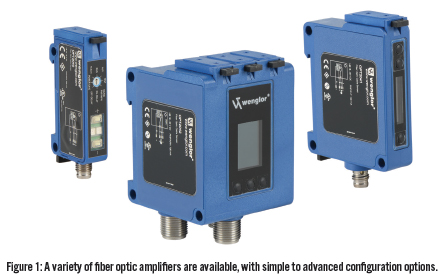
Fiber optic amplifiers range from those with basic electronics and plug-and-play functionality, to models with fully configurable electronics (Figure 1). Some even have electronic units that can handle up to 15 fiber inputs in a manifold-like configuration. Output indication is highly desirable on fiber optic electronics as it shows whether the sensor is working properly, but other basic functions, shown in Table 1, must be specified. The output format and connection to the amplifier are important because they define the interface to the controller, and teaching the on and off setpoints is an integral part of amplifier configuration.
Output types can be set normally open or normally closed; switching options include sinking, sourcing or push-pull, which allows the device to either sink or source the signal automatically depending how the circuit is wired. Electrical connection options are generally prewired with at least a 2m cable, or a quick-disconnect with a standard M8 or M12 multi-pin connector. Switch settings are programmed by dialing in a potentiometer or digitally via pushbuttons.
Beyond the basics, advanced amplifier capabilities provide significant flexibility with features such as pulse outputs, on/off delays, and the ability to eliminate intermittent signals. These advanced electronics give machine builders the ability to drill down and tweak amplifier parameters as required by the application.
On/off delays are often desired to slow the reaction of the control system to changes in sensed parameters. In the case of intermittent signals, some applications present the sensor with spurious, short-term signals which aren’t consistent with overall operating conditions. The ability to eliminate these signals at the sensor frees up the controller from this task.
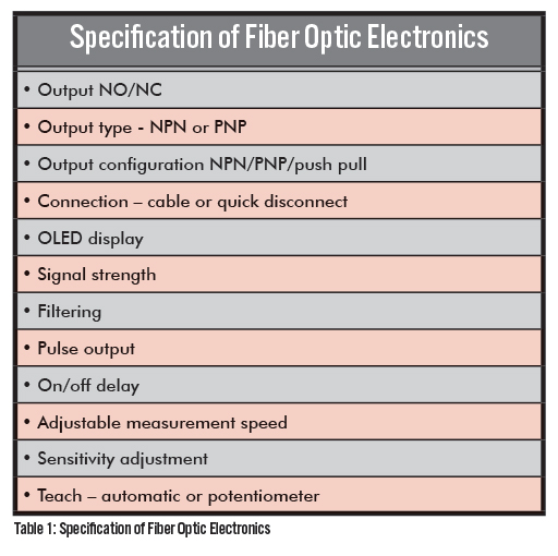
Most all models will provide output status LEDs, while some offer graduated displays to provide a coarse view of signal strength and output status. More advanced units have multiline OLED displays with customized diagnostics and programming.
Filtering is an option often needed with increased sampling rates as it provides a more resilient measurement less susceptible to ambient conditions. This stronger signal, however, requires the unit to operate at slower switching frequencies. Pulse outputs allow stretching the input signal which may help when the operating frequency is too fast for a PLC input. On/off delays give machine builders the ability to add timers when the output signal starts and stops.
Advanced units provide more programming options such as sensitivity adjustments. Using these options, machine builders can teach the machine to sense part absence, part presence or both for difficult materials like glass. This teaching function reduces or eliminates the need for programming the controller to perform these functions.
They can also set the output to switch off/on at two switch points; for example, switching on at one and off at another, such as supplying a fill level signal for a pump.
Seeing the Light with Fiber Cable
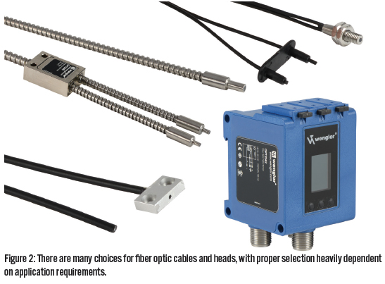
Fiber optic cables don’t conduct electricity, but instead transmit light. They come in a variety of configurations with different material types and optic head styles (Figure 2). Table 2 lists some of the decisions needed when specifying fiber optic cable.
Diffused fiber optic cables have two leads to insert in the amplifier for the emitter and receiver light, with the two leads joined together near the single optical head. Through-beam fiber optic cables are two separate, identical cables which are connected to the amplifier, each with their own optical head. One cable transmits the emitting light, and the other transmits the receiving light. A common mistake is only ordering one through-beam cable as some suppliers may provide one piece per part number, while others package the required two cables.
Fibers materials are generally either plastic or glass. Plastic units are thinner, less expensive and provide a tighter bending radius. Glass units are more rugged and can handle higher operating temperatures. Plastic fibers can be cut to length with a special one-time cutter, while glass fibers cannot be cut once received from the supplier. The fiber jacket material can also vary from a basic extruded plastic to stainless steel braiding to operate reliably in the toughest environments.
Optical head selection is the most crucial part of fiber optic sensor specification because it greatly affects the detection of the small stationary or moving parts found in most applications. Head selection differs in how the emitter and receiver optics are oriented in angle and dispersion to the object to be detected. Heads can have rounded bundles of fiber to project a circular beam, or spread out to form a horizontal, ribbon-like projection.
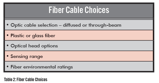
Round bundles in a diffuse head can be strictly bifurcated with all emitter fibers on one half and all receiver fibers on the other. This is common, but can cause a lag in reading a part moving perpendicular to the bifurcation line. Another option is to have the emitter and receiver fibers dispersed evenly in the head to produce a more homogenous beam. Homogenous fiber mixing gives equal exposure to sending and receiving light, and provides detection independent of part travel direction.
Sensing range for fiber optics is impacted by the amplifier, fiber cable length and type of optical head. Due to these many factors, it is usually difficult to determine an exact working range, but suppliers typically supply an estimate. Generally speaking, through-beam styles have a longer range than diffuse. The longer the fiber cable, the shorter the range; advanced amplifiers usually have stronger emitting signals and longer ranges as well.
Connecting Fiber Optic Sensors
The use of distributed I/O and distributed smart devices has been increasing throughout machine automation, and fiber optic sensors are no exception. Connecting multiple fiber optic sensor cables to a single manifold of electronics has its advantages.
Fiber optic amplifiers are commonly single-channel stand-alone units. With slim housings and common DIN rail mounting, they can easily be sandwiched and stacked in a panel. The drawback can be routing electrical connections for each of the single amplifiers.
Another option is to use a fiber optic manifold which groups multiple fiber channels to one central control and electrical point (Figure 3). These manifolds typically utilize an OLED display with menus to allow programming of each fiber channel. Each fiber channel can be configured separately, such as setting light-on or dark-on, and switching hysteresis. This central control also allows grouping of outputs via basic AND/OR logic, which can reduce and simplify the output signal to the PLC.

Applications and Issues
Fiber optics work well and are commonly used in applications where there is significant electrical noise generated by such sources as automated welding, variable frequency drives and motors. Fiber cabling is immune to electrical noise, and the electronics can be mounted away from the noise in a shielded enclosure.
Another very common application is small part assembly. These operations tend to be fully automated and thus require multiple sensors to confirm part placement (seated), and assembly verification to confirm an operation was completed. Typically, the parts are moving in and out of a stage quickly on carriers or an indexing table. There is minimal travel tolerance, so precise measurement of position
is essential.
A fiber optic solution provides various options in head size, orientation and light dispersion to allow the smallest and most accurate light focus for each application regardless of the electrical housing size. With on-board logic, one channel of a two-channel sensor can confirm a part is in place to trigger an assembly action, while the other channel can confirm that assembly was completed.
A common issue in fiber optic installations is excessive flexing of the fibers. Since the fiber cables are bundles of individual fibers, they typically feel quite pliable, allowing an installer to bend the fibers beyond their recommended maximum bend radius very easily. This can cause irrecoverable plastic deformation of the fibers, which will reduce the light transmission, or sever it entirely in the worst case. The maximum bend radius is listed with all fibers and varies depending on fiber material, bundle size and fiber dispersion in the bundle; and it must be adhered to in all cases.
Regardless of the application, machine builders must select the proper sensor technology. If fiber optic sensors are used, amplifiers and fiber optical heads must be carefully selected for the application to provide robust sensing performance.
By Andrew Waugh,
Sensor and Safety Components Product Manager, AutomationDirect
Originally Published: March 1, 2017